


Harry Cheselwoods
December 18, 2025
Share this post
Soiling loss—the reduction in PV module output caused by the accumulation of dust, pollen, and other particulates on the glass surface—remains a modelling challenge for the solar industry. Accurately modelling these losses is crucial for realistic pre-construction energy yield assessments but soiling rates are location specific, rarely consistent and hard to predict without good data.
To support more accurate, globally scaleable soiling analysis, we have added two new soiling parameters to the Solcast API. Our forecast, live, timeseries and TMY endpoints now include global data for particulate matter, specifically PM2.5 and PM10 concentrations. By integrating these parameters directly alongside our existing irradiance and weather data, we are making it easier for solar developers, asset owners, and data scientists to model real soiling, based on real data, for assets anywhere in the world.
What are PM2.5 and PM10, and why do they matter for solar?
Particulate Matter (PM) refers to a mixture of solid particles and liquid droplets found in the air. These classifications are based on particle size:
- PM10: Particulates with diameters 10 micrometres and smaller (including PM2.5).
- PM2.5: Fine particulates with diameters 2.5 micrometres and smaller (a subset of PM10).
While PM concentrations are commonly used to monitor air quality and human health impacts, in the context of solar energy, they represent the airborne materials—such as mineral dust, agricultural debris, sea salt, soot, and smoke from wildfires—that eventually settle on PV modules.
High ambient concentrations of PM2.5 and PM10 correlate with higher rates of soiling accumulation. By explicitly modelling soiling rates fora specific project location, operators can move beyond static derate factors and simulate dynamic dust accumulation and rainfall cleaning events, supporting data based cleaning planning, and more accurate loss factor modelling.
Note: Solcast PM data is intended specifically for solar soiling modelling and general analytics. It is not designed for regulatory air-quality compliance reporting.
Powered by MERRA-2 and CAMS
To ensure reliable global coverage across all time horizons, our PM data is sourced from industry-standard atmospheric monitoring
- Historic Data: Sourced from the NASA MERRA-2 reanalysis dataset.
- Live and Near-term Forecast (0–5 days): Sourced from the Copernicus Atmosphere Monitoring Service (CAMS).
- Longer-term Forecast (5–14 days): Sourced from MERRA-2 climatology.
The data is provided at an approximate spatial resolution of0.5 degrees, with temporal resolution matching your requested Solcast data—up to every 5 minutes.
Using Solcast PM data with the HSU soiling model
The HSU soiling model (Coello & Boyle 2019) is a widely used and well respected method for calculating soiling losses. Unlike simpler models, HSU accounts for spatially and temporally varying accumulation rates driven by airborne particulate matter.
The model is readily available in the open-source pvlib Python library. A typical workflow involves requesting a Solcast historic timeseries including precipitation, wind, and PM data, and feeding these inputsdirectly into the pvlib.soiling.hsu function to calculate daily soiling ratios.
Below is an example Python snippet illustrating how these inputs come together:
# Weather & irradiance
url      = f"https://api.solcast.com.au/data/historic/radiation_and_weather?latitude={latitude}&longitude=
         {longitude}&start=2025-11-01T00:00:00.000Z&&duration=P30D&period=PT60M&output_parameters=pm2.5,
         pm10,precipitation_rate&format=json"
headers  = {
    'Authorization': f'Bearer {api_key}',
    'Content-Type': 'application/json'
}

response  = requests.request("GET", url, headers=headers)

# Transform data to json
data_json = response.json()

# Transform JSON to DataFrame
df        = pd.DataFrame(data_json['estimated_actuals'])
df.index  = pd.to_datetime(df.period_end)
df.drop(["period_end"],axis=1,inplace=True)
df.index.name = None
df

pm25_gm3 = df["pm2.5"] * 1e-6
pm10_gm3 = df["pm10"] * 1e-6

tilt_deg              = 25.0
cleaning_threshold_mm = 0.5
depo_vel = {"2_5": 0.0009, "10": 0.004}  # typical defaults from the model

soiling_ratio = hsu(
    rainfall=df.precipitation_rate,                 # mm per interval
    cleaning_threshold=cleaning_threshold_mm,
    tilt=tilt_deg,                                  # degrees
    pm2_5=pm25_gm3.values,                          # g/m³
    pm10=pm10_gm3.values,                           # g/m³
    depo_veloc=depo_vel
)
What can you do with it?
By integrating PM data into your workflows, you can move from assumed soiling losses to data-driven estimates. This enables you to answer critical questions across the project lifecycle:
- What is the long-term average soiling at this location?
- Did a specific project experience excessive soiling due to wildfires?
- How does the seasonality of nearby agricultural operations lead to changes in soiling rate at my project?
- Is increased soiling causing unexpected underperformance
- How would different cleaning frequencies impact the financial return of an operational asset given its specific PM exposure?
Visualising non-local soiling events
It is important to remember that soiling is not just a local phenomenon. Particulate matter, such as desert dust or wildfire smoke, can be transported over vast distances.
The video below illustrates a significant Saharan dust plume event affecting North America in June 2020. The map shows high aerosol optical depth over the Gulf Coast. The accompanying time series for a site near Midland, Texas, shows how the arrival of this plume causes a sharp increase in the modelled soiling accumulation rate, deviating significantly from typical levels that would be returned using climatological modelling.